Data Understanding

Data Understanding¶

Welcome to the second video of the tutorial for the AI Starter Kit on remaining useful lifetime prediction! In this video, we will detail the dataset that will use and perform an initial data exploration to extract some first insights.

In this AI Starter Kit, we will work with a publicly-available dataset from NASA. The data simulates run-to-failure data from aircraft engines. These engines are assumed to start with varying degrees of wear and manufacturing variation - but this information is unknown to the user. Furthermore, in this simulated data, the engines are assumed to be operating normally at the beginning and start to degrade at some point during operation. The degradation progresses and grows in magnitude with time. When a predefined threshold is reached, the engine is considered unsafe for further operation. In other words, the last operational cycle of the engine can be considered as the failure point of the corresponding engine – meaning that the remaining useful lifetime has decreased to zero.

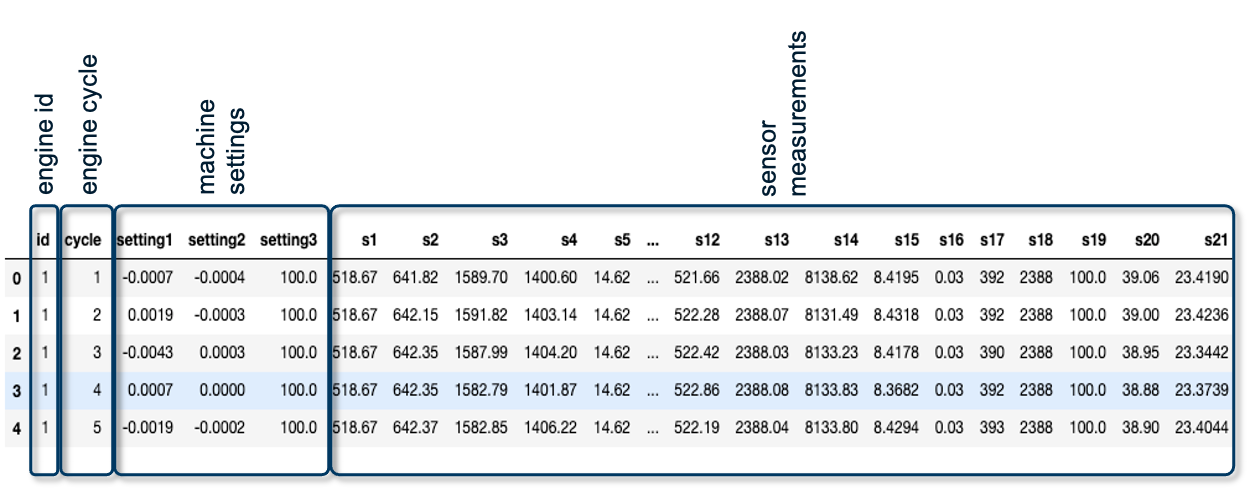
Before we can start with learning an actual machine learning model, it is crucial to understand the data itself. The data set consists of multiple time series with the "cycle" variable as time unit. For each engine, identified by the variable “id”, a different number of cycles is captured as not all engines fail at the same time. Per cycle, the following information in gathered: On the one hand, 21 sensor readings given by the data points s1 to s21. On the other hand, additional information about the machine settings, given by setting1 to setting3.

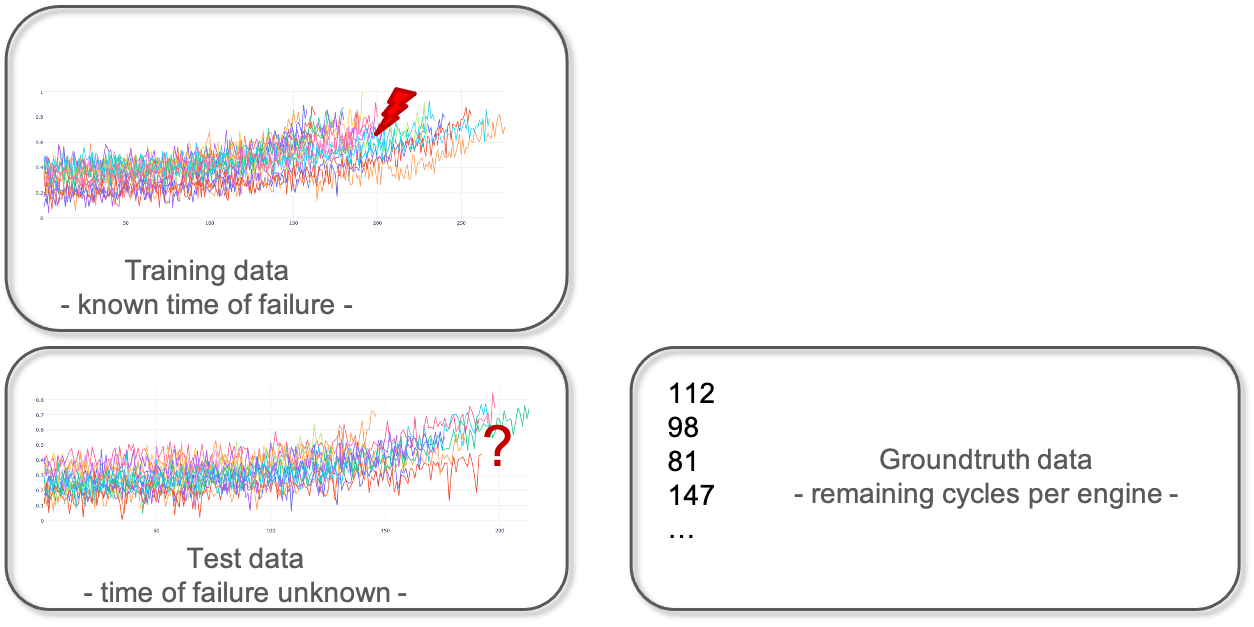
In machine learning experiments, a dataset is often split in a training set and a test set. This split allows one to quickly evaluate the performance of an algorithm. The training dataset is used to prepare a model, to train it. For evaluation, the test dataset can be understood as new data that is presented to the algorithm. It was not seen by the algorithm before and therefore the outcome is unknown. In our example, it is data from different engines for which it is unclear when they are going to fail, or put differently, what their remaining useful lifetime is. For the purpose of evaluation, the information about the actual failure of the test data set is collected in the so-called ground truth data. This information will not be visible to the algorithm but will only be used for calculating the quality of the model.

Now let’s have a look at the single sensor measurements. We see that the value range of the single measurements are quite different, without knowing in detail what they correspond to in a sense of physical measurement.

In the graph, we see the first 50 entries of time series data collected from three different sensor channels for engine 18. All three show some fluctuations but no clear deviation from a mean value indicated by the gray dotted lines, that could be a sign of degradation in engine performance, are visible. With increasing observation time, all three time series deviate more or less strongly from the mean values observed in the first 50 data points given by the gray horizontal line, indicating the start of the degradation process of the engine. For different engines, the deviation starts at different times. For engine 18, the deviation starts approximately at time 100. For engine 31 though, hardly any deviation is visible in the same time range. Only when increasing the time range, the clear deviation becomes evident. The different starting points of degradation for the single engines indicate that the simulations are made for engines with different wear.

In the next video, we will go into more detail into the data preprocessing phase, explaining how the data needs to be prepared such that it can be served as input for a machine learning learning algorithm.

If you are not familiar with deep learning, we recommend you to first watch our introductory video on this topic, in which we discuss the difference between ‘traditional’ Machine Learning algorithms and Deep Learning techniques. We will also provide a brief introduction to the different type of neural networks, amongst others the so-called Long Short-Term Memory networks or LSTMs for short, which is the type of network that we will use to solve this problem.